Pathways analysis
Now, next step is an inner join of the human biosystems table with the pivoted target table. This will add all the biosystems to which our identified proteinNameC proteins are associated altogether with an association score. This step is required to run the pathways analysis (biosystems=pathways in the context of this summary). The target table yet with the biosystems ID and biosystems name is pivoted now by biosystem keeping the count of proteins affected by compounds in each biosystem so as its average count ratio for such proteins. To the biosystems table we add proteinNameC values from the humanPathways table to get the whole amount of proteins of each biosystem. We do this through successive inner joins of Human biosystems (by biosystemsID) and Uniprot decoder table to get again the proteinNameC, but now for all existing proteins in our selected biosystems. All we have to do next is to identify these that appeared in our activities table from those that didn’t. We’ll do it through an additional join with our identified targets, either from our score selection or from Arules output. The final output of this table becomes as follows:
| Biosystem_ID | Biosystem_ID |
| source_biosystem_DB | source_biosystem_DB |
| biosystem_name | biosystem_name |
| biosystem_type | biosystem_type |
| Count(proteinNameC) for | Number of identified proteins in the biosystem |
| Avg(countRatio) for | ratio of activeprotein vs total identified protein biosystems. |
| target | Gi protein number for join |
| score | Association score of biosystem to target (by ChemBl) |
| proteinNameC | Name of the protein target |
| identifiedIn_ourTarget_Screen | If the protein is in the original dataset |
| TargetIdentifiedFromArules | If Arules identified the protein with the current confidence or support |
| BiosystemIdentifiedFromArules | If Arules identified the biosystem with the current confidence or support |
This methodology allows the identification of proteins that, despite not being present in our original dataset, play a role in the same biosystem, where the proteins we have already identified currently do, thus being candidates as members of the same signalling chain, providing similar output upon molecular intervention.
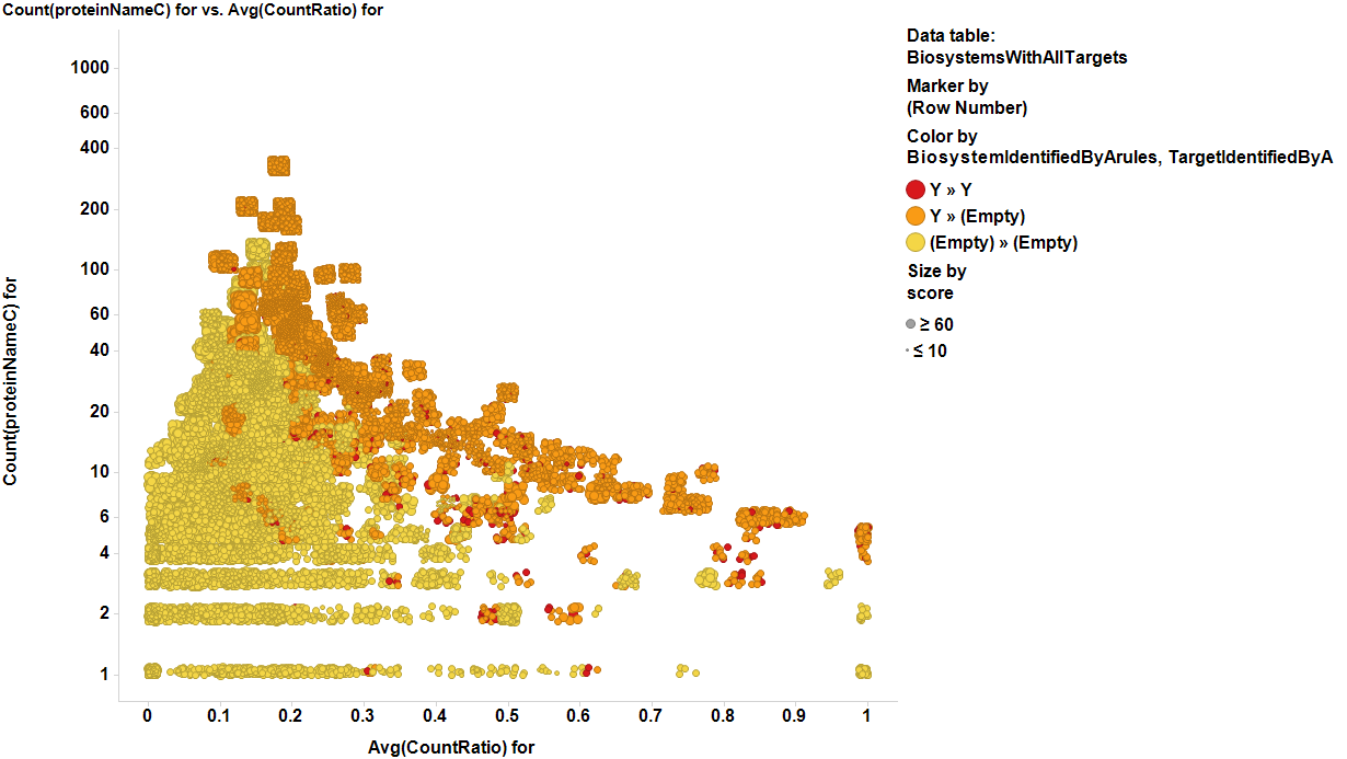
We can use identified targets to locate their pathways as described in the target selection section, and then, identify all targets of these pathways which would allow us to discriminate between known and unknown targets. Being the latest novel targets for further research. To do this, we have to calculate new indexes based on pathways. Now, countRatio is the amount of proteins in a particular active declared targets vs the total number of proteins assayed in that pathway, while countProteinNameC variable is the number of total proteins assayed in that target. With these indexes we can select the pathways with best ratios and counts using either direct estimation or a weighted function. In this work I have chosen association rules, because it gives us an estimation of acceptability of the selection based on confidence, support and lift. In the following charts we show how these plots highlight the best targets in BrCa and SMN2 models. Note that Association rules identify a small number of potential targets (red dots in the charts) but through these targets, identify most of the biosystems (orange dots), thus allowing us to mark most of the potential proteins.
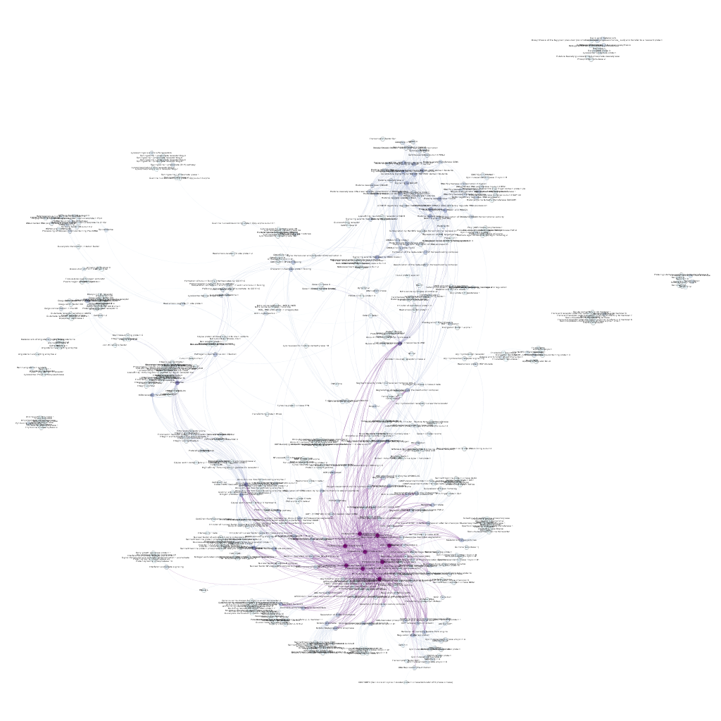
The last step is the visualization of the targets and biosystems’ relationship. To do this, we simply read the scored biosystems/protein pairs list with R to save in a gml file that we use in Gephi to build up a relationship graph.


